This is pretty easy to do with a couple of added fields to make the formulas easier.
Numbers includes a DATEDIF() function that will calculate the number of days between two dates.
For this purpose, create a new column that calculates the DATEDIF().
For example, if your Expiry Dates are in Column B, then set C1 to:
=DATEDIF(TODAY(),B1,"D")
This will calculate the difference between TODAY()'s date and the date in cell B1, and return the number of Days (denoted by the "D" parameter). Fill this formula down the column. You can optionally hide this column if you want to ignore it.
Now, in your summary table you can incorporate COUNTIF() to count the number of cells that match your criteria (less than 7 days, 8-14 days, 15-30 days) like:
Expiring in <7 days:
=COUNTIF(Table 1::C,"<=7")
COUNTIF() works by taking a range (in this case the columns of DATEDIF() values) and matches them to a condition (in this case "<=7" meaning less than or equal to 7 days).
Expiring in 8-14 days:
=COUNTIFS(Table 1::C,">7",Table 1::C,"<=14")
COUNTIFS works like COUNTIF, but supports multiple conditional checks, so we want cells that are greater than 7, AND less than/equal to 14).
Similarly, 15-30 days:
=COUNTIFS(Table 1::C,">14",Table 1::C,"<=30")
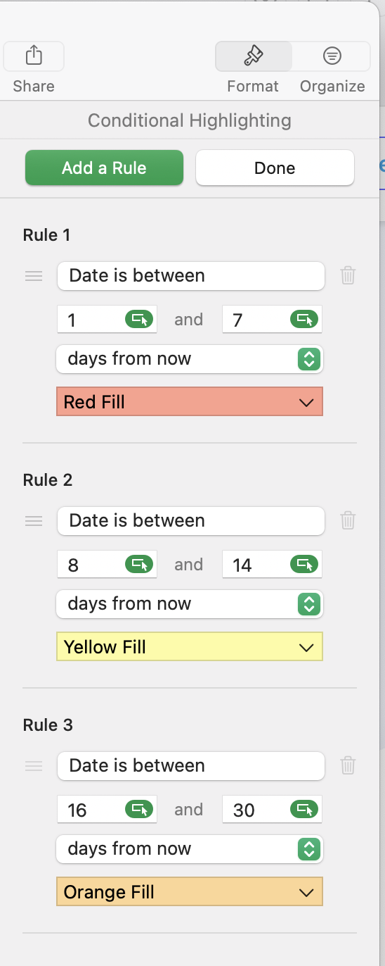
> and ideally, if it's 7 days or less till expiry, the specific account's Expiry Date cell (below) would turn red; if 8–14 days till expiry, the cell would turn yellow; if 15–30 days till expiry, the cell would turn orange.
The formatting is even easier - Numbers can do this automatically.
Just select the date cells and choose Inspector -> Format -> Cell and click the Conditional Hightlighing button.
Numbers can use a number of conditions to set the formatting. In this case choose Date functions and the 'Date is Between...' option.
You can set the number of days to check and what format to apply when the conditions match. Here's an example:
