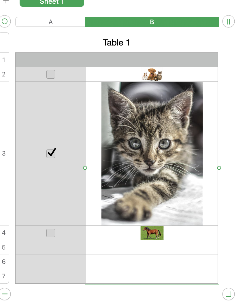
That's pretty good. It made me think of the idea below where the images don't have to be in two places.

Formula in all data cells of column B (with the images) is =IF(A,REPT(CHAR(8232),15),"")
This creates a string of 15 line separator characters when the checkbox is checked. If the row heights are the default "automatic fit", the row height will expand. Use something larger than 15 to get a larger image. The width of column B will limit its size. Wider column = ability to show a larger image.
If the database is already populated with images you won't be able to drag-fill the formula to get the formula in all the rows. It will drag-fill the image along with it. You will have to copy/paste.
- Copy the formula from here, including the equals sign
- Select all the data cells in column B,
- Paste
If you want to edit them later (such as to change the 15 to something else),
- Edit one of them,
- Copy that cell,
- Paste & Match Style to the rest of the column. Do not use the normal Paste.
To "scroll" through the images/rows you can do this
- Select one of the checkbox cells
- Space bar to check it
- Space bar to uncheck it
- Arrow key to move to the next row
- Repeat at 2