Formula or template for calculation

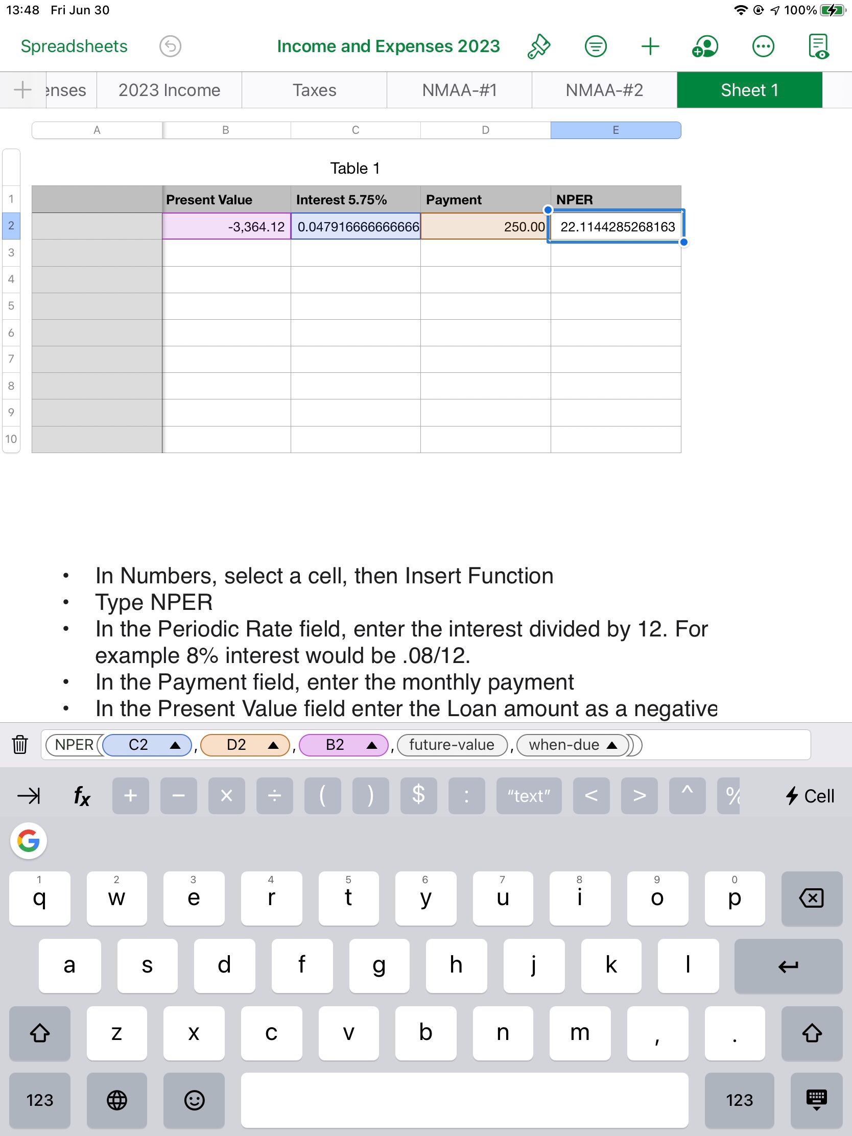
Ok, I followed what you said but I don't I understand about the NPER cell.

I entered NPER in the last column, first row which is E2.

That resulted in a formula with descriptive labels.

I replaced the 3 of the descriptive labels with the cells as follows:

1. For the "periodic-rate" value label I replaced it with C2 which is 5.75% (entered as 0.575/12) and the cell converted it to 0.04791666...
2. For the "payment" value label, I replaced it with D2 which is $250.00
3. For "present-value" label I replaced it with B2 which is the loan balance in a negative (-$3,364.12)

I then backed out of cell E2 and it automatically calculated 22.114428....

When I clicked back on cell E2 there are still 2 descriptivelabels, "future-value" and "when-due".

I think column E is showing me the number of months it would take to pay down the loan.

Do I just ignore those other 2 descriptive labels in the formula for cell E2? Or remove them from the formula?

Is NPER something that is versatile? Meaning in the future I can use it in tables to determine any unknown by substituting each descriptive label with a specific cell of known data and then ignore or delete the other descriptive labels that don't apply?

I am guessing if I set up a column with a payment date on the 20th of July, I would replace "when-due" with the cell containing the payment date. Or if I set up a column of the balance after a payment, I would replace "future-balance" with that cell.

Again, I appreciate the formula which I think is showing me it will take about 22 months to pay off about $3,364 at 5.75% interest, if I pay $250 each month.

I just started using Numbers a couple of months ago to set up a budget. I've Numbers for years and know about linking cells in table and simple Totals for a column or row but I've not dealt with formulas until now.

Thanks very much!

Great information!! I'm going to chunk out some time blocks to study your linked info. I also enrolled in a Mac Most Numbers course. A bit dated but still seems pertinent to help me visualize the things Numbers is capable of.

Thanks, but I did visit the available Templates, Apple Support and the Numbers Help menu before posting my question. None of them explained what I needed in a way I could understand. The information they presented was just too overwhelming to comprehend as it was far beyond my experience level.

Mac Jim ID provided the exact formula I needed. His answer allowed me to understand how the descriptive labels are used in regards to cells so that the formula/function can solve the unknown. Applying that one formula to my situation is what really helped my brain make sense of the "nonsense" that I was seeing whenever I typed in a formula/function that I found on Apple Support.

I know you will laugh, but I did try entering NPER and hitting Enter. Nothing happened. That's because I didn't know that I needed to assign cells to the labels!!!!

The built in Numbers templates don't calculate loan amorization in regards to determining payment amounts over varous periods of time. I've explored them many times, but I haven't found a use for them yet. I opened them all again yesterday but I havent found any I need.

I wasn't able to find any videos in the Apple Support area. If you do know of any Apple Support videos please let me know. Trying to comprehend the written explanations in Apple Support or Numbers Help just brings on frustration.

I am sure at some point the written information in the Help menu will come in handy. They seem geared more to a user who already understands the definition and purpose of a formula/function. I am not quite up to that level yet.

I knew an entire numerical column could be used to add or subtract to reach a total but I was unaware that individual cells could be selected regardless of where they were located to solve for so many different unknowns. I don't have a background in mathematical terminology or the manipulation of numbers.

The MacMost Numbers video course by Gary Rosenzweig uses examples to demonstrate the impact of various formulas. The interactive video format is helping me grasp how to connect the correct cell to a descriptive label in a formula/function. I'm not sure I understand yet how a formula is different from a function.

Thanks for suggestions and I'll keep them in mind. I am sure they will help as a reference and make more sense what I get a better grasp on the subject.

Yes he does have a lot of vids free on you tube but his Numbers course is only available through his Mac Most site and Udemy. His YT vids are just a few of the bits and pieces of his complete course. The Udemy site has the same syllabus as the Mac Most site. He's a great instructor. I've taken other courses of his on Pages, Keynote, iMovie and Final Cut.

Being able to start from the beginning and work all the modules of Numbers from beginning to end is something I find of value to pay for. (The YT vids leave it up to the user to pick and choose specific learning points which I got lost in.)

I've only recently had the desire to use Numbers for retirement scenarios and tax planning situations in which one of us outlives the other. Up until now I've just used it to compile sums for our CPA. But now I want to use Numbers for financial planning strategies. (Our investment advisor has a lot of online tools and their website compiles the investments we already have in place.) While I have great trust in my Financial Management Advisor (a small local family business) I want to explore and take on a more active role to increase my understanding.

I'm suppose I am in the "next phase" of using/understanding Numbers. I'm now retired with more time on my hands. I want to run some figures on spend down scenarios, payoff scenarios and possibly building up funds in an annuity as a tax deferred vehicle the other spouse would inherit. Or our children.

My last involvement with databases and spreadsheets was in '95-96 during a post grad research course and internship. Just two classes and the focus was health care research, not finance or business accounting. And it was on Unix and PCs.

Thanks for your helpful insights.

Many thanks!